Zero-order Gradient Differentiation
Evolutionary Strategy

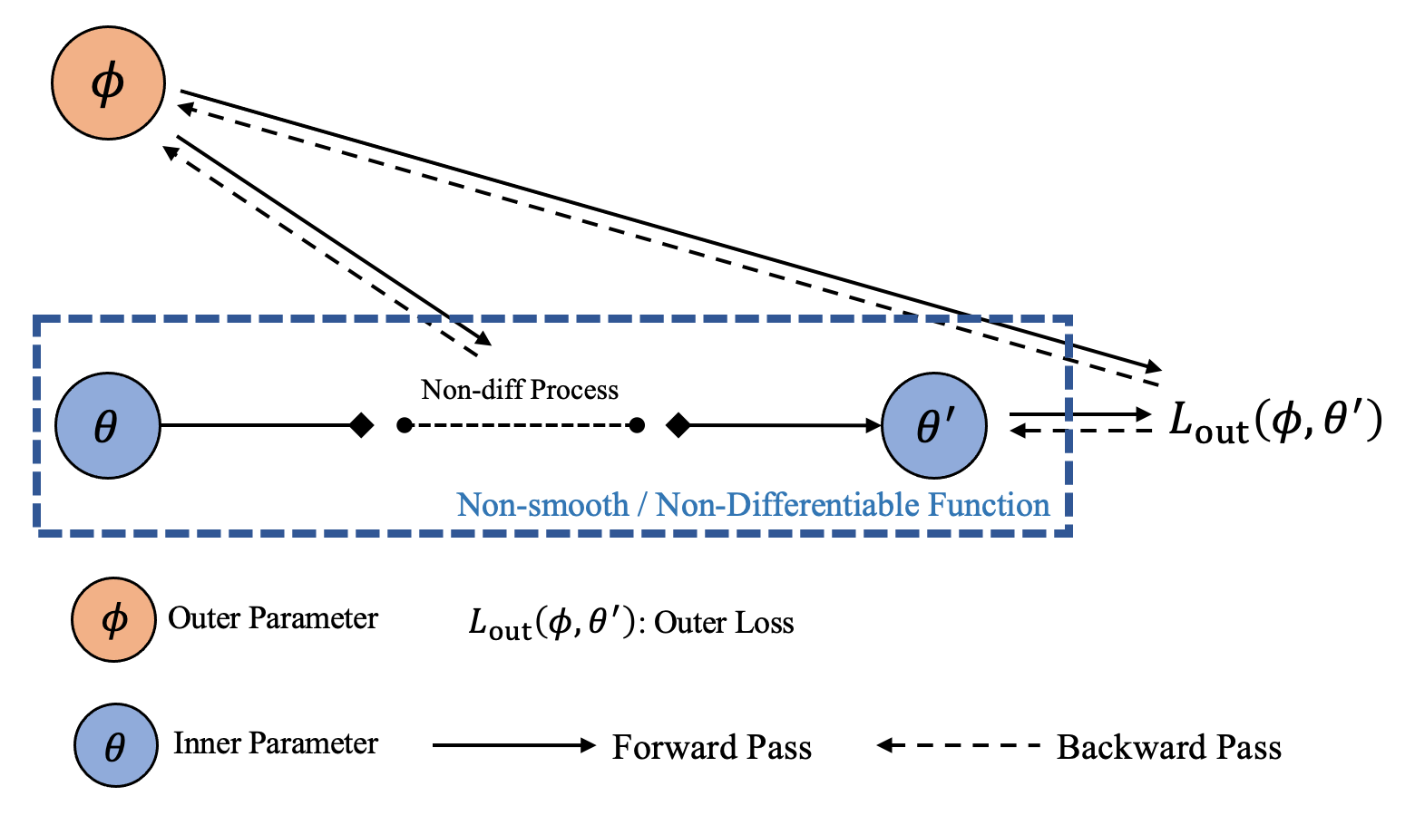
When the inner-loop process is non-differentiable or one wants to eliminate the heavy computation burdens in the previous two modes (brought by Hessian), one can choose Zeroth-order differentiation. Zero-order differentiation typically gets gradients based on zero-order estimation, such as finite-difference, or Evolutionary Strategy (ES). ES-MAML and NAC successfully solve the non-differentiable optimization problem based on ES.
TorchOpt offers API for ES-based differentiation. Instead of optimizing the objective \(f (\boldsymbol{\theta}): \mathbb{R}^n \to \mathbb{R}\), ES optimizes a Gaussian smoothing objective defined as \(\tilde{f}_{\sigma} (\boldsymbol{\theta}) = \mathbb{E}_{\boldsymbol{z} \sim \mathcal{N}( 0, {I}_d )} [ f (\boldsymbol{\theta} + \sigma \, \boldsymbol{z}) ]\), where \(\sigma\) denotes the precision. The gradient of such objective is \(\nabla_{\boldsymbol{\theta}} \tilde{f}_{\sigma} (\boldsymbol{\theta}) = \frac{1}{\sigma} \mathbb{E}_{\boldsymbol{z} \sim \mathcal{N}( 0, {I}_d )} [ f (\boldsymbol{\theta} + \sigma \, \boldsymbol{z}) \cdot \boldsymbol{z} ]\). Based on such technique, one can treat the bi-level process as a whole to calculate the meta-gradient based on pure forward process. Refer to ES-MAML for more explanations.
Decorators
|
Return a decorator for applying zero-order differentiation. |
Similar to the implicit gradient, we also use the decorator for ES methods.
Functional API
The basic functional API is torchopt.diff.zero_order.zero_order(), which is used as the decorator for the forward process zero-order gradient procedures.
Users are required to implement the noise sampling function, which will be used as the input of the zero_order decorator.
Here we show the specific meaning for each parameter used in the decorator.
distributionfor noise sampling distribution. The distribution \(\lambda\) should be spherical symmetric and with a constant variance of \(1\) for each element. I.e.:Spherical symmetric: \(\mathbb{E}_{\boldsymbol{z} \sim \lambda} [ \boldsymbol{z} ] = \boldsymbol{0}\).
Constant variance of \(1\) for each element: \(\mathbb{E}_{\boldsymbol{z} \sim \lambda} [ {\lvert z_i \rvert}^2 ] = 1\).
For example, the standard multi-dimensional normal distribution \(\mathcal{N} (\boldsymbol{0}, \boldsymbol{1})\).
methodfor different kind of algorithms, we support'naive'(ES RL),'forward'(Forward-FD), and'antithetic'(antithetic).\[\begin{align*} \text{naive} \qquad & \nabla_{\boldsymbol{\theta}} \tilde{f}_{\sigma} (\boldsymbol{\theta}) = \frac{1}{\sigma} \mathbb{E}_{\boldsymbol{z} \sim \lambda} [ f (\boldsymbol{\theta} + \sigma \, \boldsymbol{z}) \cdot \boldsymbol{z} ] \\ \text{forward} \qquad & \nabla_{\boldsymbol{\theta}} \tilde{f}_{\sigma} (\boldsymbol{\theta}) = \frac{1}{\sigma} \mathbb{E}_{\boldsymbol{z} \sim \lambda} [ ( f (\boldsymbol{\theta} + \sigma \, \boldsymbol{z}) - f (\boldsymbol{\theta}) ) \cdot \boldsymbol{z} ] \\ \text{antithetic} \qquad & \nabla_{\boldsymbol{\theta}} \tilde{f}_{\sigma} (\boldsymbol{\theta}) = \frac{1}{2 \sigma} \mathbb{E}_{\boldsymbol{z} \sim \lambda} [ (f (\boldsymbol{\theta} + \sigma \, \boldsymbol{z}) - f (\boldsymbol{\theta} + \sigma \, \boldsymbol{z}) ) \cdot \boldsymbol{z} ] \end{align*}\]argnumsspecifies which parameter we want to trace the meta-gradient.num_samplesspecifies how many times we want to conduct the sampling.sigmais for precision. This is the scaling factor for the sampling distribution.
We show the pseudo code in the following part.
# Functional API for zero-order differentiation
# 1. Customize the noise distribution via a distribution class
class Distribution:
    def sample(self, sample_shape=torch.Size()):
        # Sampling function for noise
        # NOTE: The distribution should be spherical symmetric and with a constant variance of 1.
        ...
        return noise_batch

distribution = Distribution()

# 2. Customize the noise distribution via a sampling function
def distribution(sample_shape=torch.Size()):
    # Sampling function for noise
    # NOTE: The distribution should be spherical symmetric and with a constant variance of 1.
    ...
    return noise_batch

# 3. Distribution can also be an instance of `torch.distributions.Distribution`, e.g., `torch.distributions.Normal(...)`
distribution = torch.distributions.Normal(loc=0, scale=1)

# Decorator that wraps the function
@torchopt.diff.zero_order(distribution=distribution, method='naive', argnums=0, num_samples=100, sigma=0.01)
def forward(params, data):
    # Forward optimization process for params
    ...
    return objective  # the returned tensor should be a scalar tensor

# Define params and get data
params, data = ..., ...

# Forward pass
loss = forward(params, data)
# Backward pass using zero-order differentiation
grads = torch.autograd.grad(loss, params)
OOP API
|
The base class for zero-order gradient models. |
Coupled with PyTorch torch.nn.Module, we also design the OOP API nn.ZeroOrderGradientModule for ES.
The core idea of nn.ZeroOrderGradientModule is to enable the gradient flow forward process to self.parameters() (can be the meta-parameters when calculating meta-gradient).
Users need to define the forward process zero-order gradient procedures forward() and a noise sampling function sample().
from torchopt.nn import ZeroOrderGradientModule

# Inherited from the class ZeroOrderGradientModule
# Optionally specify the `method` and/or `num_samples` and/or `sigma` used for sampling
class Net(ZeroOrderGradientModule, method='naive', num_samples=100, sigma=0.01):
    def __init__(self, ...):
        ...

    def forward(self, batch):
        # Forward process
        ...
        return objective  # the returned tensor should be a scalar tensor

    def sample(self, sample_shape=torch.Size()):
        # Generate a batch of noise samples
        # NOTE: The distribution should be spherical symmetric and with a constant variance of 1.
        ...
        return noise_batch

# Get model and data
net = Net(...)
data = ...

# Forward pass
loss = Net(data)
# Backward pass using zero-order differentiation
grads = torch.autograd.grad(loss, net.parameters())
Notebook Tutorial
For more details, check the notebook tutorial at zero-order.