Implicit Gradient Differentiation
Implicit Differentiation
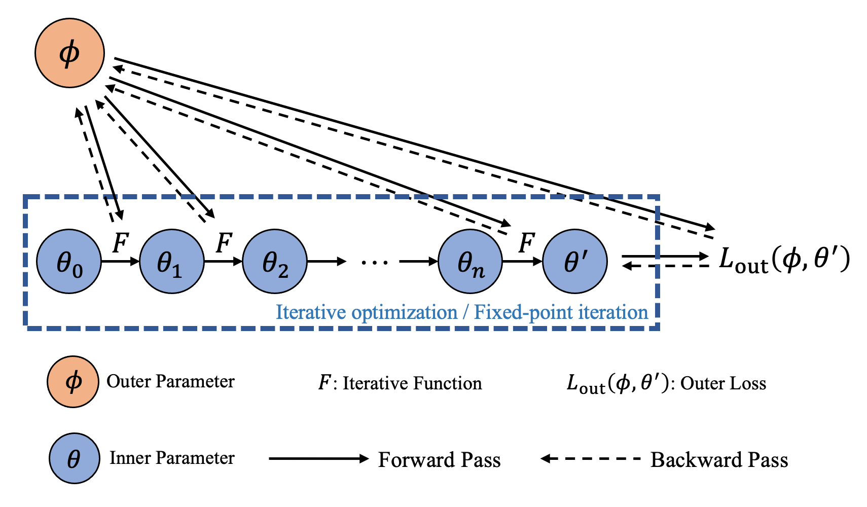
Implicit differentiation is the task of differentiating through the solution of an optimization problem satisfying a mapping function \(T\) capturing the optimality conditions of the problem. The simplest example is to differentiate through the solution of a minimization problem with respect to its inputs. Namely, given
By treating the solution \(\boldsymbol{\theta}^{\prime}\) as an implicit function of \(\boldsymbol{\phi}\), the idea of implicit differentiation is to directly get analytical best-response derivatives \(\nabla_{\boldsymbol{\phi}} \boldsymbol{\theta}^{\prime} (\boldsymbol{\phi})\) by the implicit function theorem.
Root Finding
This is suitable for algorithms when the inner-level optimality conditions \(T\) is defined by a root of a function, such as:
In IMAML, the function \(F\) in the figure means the inner-level optimal solution is obtained by unrolled gradient update:
Fixed-point Iteration
Sometimes the inner-level optimal solution can also be achieved by fixed point where the optimality \(T\) takes the form:
In DEQ, the function \(F\) in the figure means the inner-level optimal solution is obtained by fixed point update:
This can be seen as a particular case of root of function by defining the optimality function as \(T (\boldsymbol{\phi}, \boldsymbol{\theta}) = F (\boldsymbol{\phi}, \boldsymbol{\theta}) - \boldsymbol{\theta}\). This can be implemented with:
def fixed_point_function(phi: TensorTree, theta: TensorTree) -> TensorTree:
    ...
    return new_theta

# A root function can be derived from the fixed point function
def root_function(phi: TensorTree, theta: TensorTree) -> TensorTree:
    new_theta = fixed_point_function(phi, theta)
    return torchopt.pytree.tree_sub(new_theta, theta)
Custom Solvers
|
Return a decorator for adding implicit differentiation to a root solver. |
Let \(T (\boldsymbol{\phi}, \boldsymbol{\theta}): \mathbb{R}^n \times \mathbb{R}^d \to \mathbb{R}^d\) be a user-provided mapping function, that captures the optimality conditions of a problem. An optimal solution, denoted \(\boldsymbol{\theta}^{\prime} (\boldsymbol{\phi})\), should be a root of \(T\):
We can see \(\boldsymbol{\theta}^{\prime} (\boldsymbol{\phi})\) as an implicitly defined function of \(\boldsymbol{\phi} \in \mathbb{R}^n\), i.e., \(\boldsymbol{\theta}^{\prime}: \mathbb{R}^n \rightarrow \mathbb{R}^d\). More precisely, from the implicit function theorem, we know that for \((\boldsymbol{\phi}_0, \boldsymbol{\theta}^{\prime}_0)\) satisfying \(T (\boldsymbol{\phi}_0, \boldsymbol{\theta}^{\prime}_0) = \boldsymbol{0}\) with a continuously differentiable \(T\), if the Jacobian \(\nabla_{\boldsymbol{\theta}^{\prime}} T\) evaluated at \((\boldsymbol{\phi}_0, \boldsymbol{\theta}^{\prime}_0)\) is a square invertible matrix, then there exists a function \(\boldsymbol{\theta}^{\prime} (\cdot)\) defined on a neighborhood of \(\boldsymbol{\phi}_0\) such that \(\boldsymbol{\theta}^{\prime} (\boldsymbol{\phi}_0) = \boldsymbol{\theta}^{\prime}_0\). Furthermore, for all \(\boldsymbol{\phi}\) in this neighborhood, we have that \(T (\boldsymbol{\phi}_0, \boldsymbol{\theta}^{\prime}_0) = \boldsymbol{0}\) and \(\nabla_{\boldsymbol{\phi}} \boldsymbol{\theta}^{\prime} (\boldsymbol{\phi})\) exists. Using the chain rule, the Jacobian \(\nabla_{\boldsymbol{\phi}} \boldsymbol{\theta}^{\prime}(\boldsymbol{\phi})\) satisfies:
Computing \(\nabla_{\boldsymbol{\phi}} \boldsymbol{\theta}^{\prime}(\boldsymbol{\phi})\) therefore boils down to the resolution of the linear system of equations
TorchOpt provides a decorator function custom_root(), for easily adding implicit differentiation on top of any existing inner optimization solver (also called forward optimization).
The custom_root() decorator requires users to define the stationary conditions for the problem solution (e.g., KKT conditions) and will automatically calculate the gradient for backward gradient computation.
Here is an example of the custom_root() decorators, which is also the functional API for implicit gradient.
# Functional API for implicit gradient
def stationary(params, meta_params, data):
    # stationary condition construction
    return stationary condition

# Decorator that wraps the function
# Optionally specify the linear solver (conjugate gradient or Neumann series)
@torchopt.diff.implicit.custom_root(stationary)
def solve(params, meta_params, data):
    # Forward optimization process for params
    return optimal_params

# Define params, meta_params and get data
params, meta_prams, data = ..., ..., ...
optimal_params = solve(params, meta_params, data)
loss = outer_loss(optimal_params)

meta_grads = torch.autograd.grad(loss, meta_params)
OOP API
|
The base class for differentiable implicit meta-gradient models. |
Coupled with PyTorch torch.nn.Module, we also design the OOP API nn.ImplicitMetaGradientModule for implicit gradient.
The core idea of nn.ImplicitMetaGradientModule is to enable the gradient flow from self.parameters() (usually lower-level parameters) to self.meta_parameters() (usually the high-level parameters).
Users need to define the forward process forward(), a stationary function optimality() (or objective()), and inner-loop optimization solve.
Here is an example of the OOP API.
from torchopt.nn import ImplicitMetaGradientModule

# Inherited from the class ImplicitMetaGradientModule
class InnerNet(ImplicitMetaGradientModule):
    def __init__(self, meta_module):
        ...

    def forward(self, batch):
        # Forward process
        ...

    def optimality(self, batch, labels):
        # Stationary condition construction for calculating implicit gradient
        # NOTE: If this method is not implemented, it will be automatically derived from the
        # gradient of the `objective` function.
        ...

    def objective(self, batch, labels):
        # Define the inner-loop optimization objective
        # NOTE: This method is optional if method `optimality` is implemented.
        ...

    def solve(self, batch, labels):
        # Conduct the inner-loop optimization
        ...
        return self  # optimized module

# Get meta_params and data
meta_params, data = ..., ...
inner_net = InnerNet()

# Solve for inner-loop process related to the meta-parameters
optimal_inner_net = inner_net.solve(meta_params, *data)

# Get outer-loss and solve for meta-gradient
loss = outer_loss(optimal_inner_net)
meta_grad = torch.autograd.grad(loss, meta_params)
If the optimization objective is to minimize/maximize an objective function, we offer an objective method interface to simplify the implementation.
Users only need to define the objective method, while TorchOpt will automatically analyze it for the stationary (optimality) condition from the KKT condition.
Note
In __init__ method, users need to define the inner parameters and meta-parameters.
By default, nn.ImplicitMetaGradientModule treats all tensors and modules from the method inputs as self.meta_parameters() / self.meta_modules().
For example, statement self.yyy = xxx will assign xxx as a meta-parameter with name 'yyy' if xxx is present in the method inputs (e.g., def __init__(self, xxx, ...): ...).
All tensors and modules defined in the __init__ are regarded as self.parameters() / self.modules().
Users can also register parameters and meta-parameters by calling self.register_parameter() and self.register_meta_parameter() respectively.
Linear System Solvers
|
Return a solver function to solve |
|
Return a solver function to solve |
|
Return a solver function to solve |
Usually, the computation of implicit gradient involves the computation of the inverse Hessian matrix. However, the high-dimensional Hessian matrix also makes direct computation intractable, and this is where linear solver comes into play. By iteratively solving the linear system problem, we can calculate the inverse Hessian matrix up to some precision. We offer the conjugate-gradient based solver and neuman-series based solver.
Here is an example of the linear solver.
import torch
from torchopt import linear_solve

torch.manual_seed(42)
A = torch.randn(3, 3)
b = torch.randn(3)

def matvec(x):
    return  torch.matmul(A, x)

solve_fn = linear_solve.solve_normal_cg(atol=1e-5)
solution = solve_fn(matvec, b)
print(solution)

solve_fn = linear_solve.solve_cg(atol=1e-5)
solution = solve_fn(matvec, b)
print(solution)
Users can also select the corresponding solver in functional and OOP APIs.
# For functional API
@torchopt.diff.implicit.custom_root(
    functorch.grad(objective_fn, argnums=0),  # optimality function
    argnums=1,
    solve=torchopt.linear_solve.solve_normal_cg(maxiter=5, atol=0),
)
def solve_fn(...):
    ...

# For OOP API
class InnerNet(
    torchopt.nn.ImplicitMetaGradientModule,
    linear_solve=torchopt.linear_solve.solve_normal_cg(maxiter=5, atol=0),
):
    ...
Notebook Tutorial
Check the notebook tutorial at Implicit Differentiation.